The Ladder of Causation

Pearl was once all for a purely probabilistic model of causality. Then one day he was climbing the ladder to his mezzanine henhouse (Jews have to raise their own hens because Jews), one hook broke and he fell down banging his head badly on the floor. It was reported that, during the trip to the hospital, he grumbled continuously half-unconscious “THE LADDER, THE LADDAHER…” He was kept in intensive care for one week. On the morning of the seventh day, he woke up and stood. The nurse got mad, put him back down on the bed and called the doctors. All the doctors came around him, who was still on the bed but had raised his back and was sitting against the headboard. He looked at them wearing his typical sly smile. The doctors asked how he felt, and thus he spoke: “THE LADDER IS THE CAUSE. THE CAUSE IS THE LADDER. ONLY AT THE TOP OF THE LADDER THE EFFECT SUCCEEDS THE CAUSE. THE CAUSE IS AT THE TOP OF THE LADDER. THE LADDER IS A LADDER OF CAUSATION.”

Mr. Pearl, how do you do? Can you look at my hand?

I SHALL LOOK.

Good. Now tell me, given that the ratio of patients hospitalized for head injury to the other patients is 1:200, and that the probability of failing the medical finger count test after a head trauma is 10 times the one in normal conditions, and that I’m showing you two fingers, what is the probability that you banged your head?

Pearl was still smiling. He clenched the doctor’s hand and broke all his fingers.

Seriously version

Seriously, you still wasting time, Rubin? Can you get your act together at last, please? Do you think that the Nobel to Imbens saves your sorry mustache? You would just need for once to compute, step by step, the probability that the identity of your father is correct, and you would immediately recognize the usefulness of causal diagrams. The light would shine through the equations.

Serious version

Pearl begins his book with the Genesis:

I was probably six or seven years old when I first read the story of Adam and Eve in the Garden of Eden. My classmates and I were not at all surprised by God’s capricious demands, forbidding them to eat from the Tree of Knowledge. Deities have their reasons, we thought. What we were more intrigued by was the idea that as soon as they ate from the Tree of Knowledge, Adam and Eve became conscious, like us, of their nakedness.

Of course the Old Testament, as a good and proper sacred text, already embodies all truths, and in particular proves Pearl right on his theories. (Is Jesus a redundant set of parameters? Or is Jesus an even more compact representation of the Truth?) Anyway, after a biblical tour, Pearl lands us on the Ladder of Causation. The Ladder has three rungs, which correspond to increasing abilities of an intelligent agent in the manipulation of causality.

Rung one is the ability to see, to observe relations and associations between things. Probabilistic reasoning belongs here: I notice that of all the times A happens, in a fraction p of those, B follows A. Then I say that p is the probability of B conditional on A, P(B|A) = p, and, if I see A again, I predict that B will happen with probability p. Every Monday, school finishes one hour earlier than usual, and you have to go home on foot. Sometimes, as soon as your house is in sight, you see a group of men rushing out from the backyard. Thus you estimate

Rung two is the ability to do. Instead of waiting for A to happen naturally, you force it to be true somehow, and compute again the probability of B given having done A, P(B|Â), where  (A with a hat) is a shorthand for the proposition “A is true, but not by the usual mechanism left implicit in the initial definition of A, but by some other mechanism I employ to make it surely true in a specific case.” An equivalent notation is P(B|do(A)), which earns it the fancy name “do-operator.” Depending on what was the original process that brought about A, this probability may be different from P(B|A). To investigate the provenance of the odd evasive folks, you decide to come back one hour earlier on Tuesday. Intuitively, this will tell you if the point is the weekday (Monday) or coming back before time. The point being that the point is the cause. You give an excuse to the principal and head home. This time you don’t notice any strangers escaping, but your mother seems very worried about your anticipated exit.

«My little mouse, how can you be home so early? It is not Monday, isn’t it?»

«Mmm nothing mom, I just… I got a very strong headache, I think I played too many video games yesterday night, and the teacher was kind and let me go home earlier.»

«Oh dear! But the school must call me before they let you out! They are mandated to confirm permission with the parents!»

«Listen mom don’t make a case of it, anyway I already feel better, don’t worry, I took two aspirins»

«Yes yes but how dare they send you out earlier in this way without informing me beforehand! This is utterly unacceptable! I must request a personal colloquy with every teacher!»

«Please mom no, it’s embarrassing, mmmalso I gave an excuse to the teacher, don’t tell them I was at the console until 3 am, teachers are so finicky about this stuff…»

“But I can’t let this thing pass! It is against the rules! I’m completely positive that this is against all the rules!»

«Mom I know you are anxious but the’re no dangers around here, ok? Like, I do it every Monday, it doesn’t change if you don’t know that I’m out, I’m fine»

«I can see very well that you are fine! But you can’t get home early without telling me first!»

Rung three is the ability to imagine. You know that A happened, followed by B. But… would B have happened if A had not? Notice this is not the probability of B given not-A, P(B|¬A), neither the probability of B given making A not happen, P(B|do(¬A)). You already know that, in the case at hand, A is true and B too, and you didn’t lift a finger to call for A. The fact that they turned out to be true could change your assessment of what would have happened in that specific circumstance if A was forced to be false. So you need to imagine not just something you don’t know, but something which contradicts your factual knowledge. This kind of thinking is called counterfactual. Your mother is again a deep source of examples, left as exercise to the reader.

Mother-free and any gender-relatable concept-free this time I promise version

So, the ladder of causation… without mothers? Whatever. Well, the ladder is not just a way to hang three concepts on a wall to satisfy the rule of three, it implies a hierarchy. (A rungarchy?) To move up one rung in the ladder, you need new mental tools and concepts that weren’t required to find your way around in the lower rung. Pearl relates this to the level of general intelligence:

So far I may have given the impression that the ability to organize our knowledge of the world into causes and effects was monolithic and acquired all at once. In fact, my research on machine learning has taught me that a causal learner must master at least three distinct levels of cognitive ability: seeing, doing, and imagining.

The first, seeing or observing, entails detection of regularities in our environment and is shared by many animals as well as early humans before the Cognitive Revolution. The second, doing, entails predicting the effect(s) of deliberate alterations of the environment and choosing among these alterations to produce a desired outcome. Only a small handful of species have demonstrated elements of this skill. Use of tools, provided it is intentional and not just accidental or copied from ancestors, could be taken as a sign of reaching this second level. Yet even tool users do not necessarily possess a “theory” of their tool that tells them why it works and what to do when it doesn’t. For that, you need to have achieved a level of understanding that permits imagining. It was primarily this third level that prepared us for further revolutions in agriculture and science and led to a sudden and drastic change in our species’ impact on the planet.

I cannot prove this, but I can prove mathematically that the three levels differ fundamentally, each unleashing capabilities that the ones below it do not.

The emphasis is mine. Elaborating further on this, Pearl explains he sees current statistics/machine learning research as stuck on rung one:

The successes of deep learning have been truly remarkable and have caught many of us by surprise. Nevertheless, deep learning has succeeded primarily by showing that certain questions or tasks we thought were difficult are in fact not [come on man!]. It has not addressed the truly difficult questions that continue to prevent us from achieving humanlike AI. As a result the public believes that “strong AI,” machines that think like humans, is just around the corner or maybe even here already. In reality, nothing could be farther from the truth. I fully agree with Gary Marcus, a neuroscientist at New York University, who recently wrote in the New York Times that the field of artificial intelligence is “bursting with microdiscoveries”—the sort of things that make good press releases—but machines are still disappointingly far from humanlike cognition. My colleague in computer science at the University of California, Los Angeles, Adnan Darwiche, has titled a position paper “Human-Level Intelligence or Animal-Like Abilities?” which I think frames the question in just the right way. The goal of strong AI is to produce machines with humanlike intelligence, able to converse with and guide humans. Deep learning has instead given us machines with truly impressive abilities but no intelligence. The difference is profound and lies in the absence of a model of reality.

Just as they did thirty years ago, machine learning programs (including those with deep neural networks) operate almost entirely in an associational mode. They are driven by a stream of observations to which they attempt to fit a function, in much the same way that a statistician tries to fit a line to a collection of points. Deep neural networks have added many more layers to the complexity of the fitted function, but raw data still drives the fitting process. They continue to improve in accuracy as more data are fitted, but they do not benefit from the “super-evolutionary speedup.” If, for example, the programmers of a driverless car want it to react differently to new situations, they have to add those new reactions explicitly. The machine will not figure out for itself that a pedestrian with a bottle of whiskey in hand is likely to respond differently to a honking horn. This lack of flexibility and adaptability is inevitable in any system that works at the first level of the Ladder of Causation.

So, Pearl has a three-bullet model of reality that explains evolution and the secret to artificial general intelligence? I think I’m starting to hear the knocks of a hammer… Ah wait that’s Ukraine’s invasion. But then tell me, when was the last time that a baby Jew geezer changed our foundational understanding of the world with a few simple equations? Ah it happens every time you say? Cool, I’ll try to be more sympathetic then. Maybe Pearl, when he says that he has proven mathematically that the three levels differ fundamentally, is just trying to churn out a convincing prose. What’s his say on this?

Decades’ worth of experience with these kinds of questions has convinced me that, in both a cognitive and a philosophical sense, the idea of causes and effects is much more fundamental than the idea of probability.

[...]

The recognition that causation is not reducible to probabilities has been very hard-won, both for me personally and for philosophers and scientists in general.

[...]

However, in their effort to mathematize the concept of causation—itself a laudable idea—philosophers were too quick to commit to the only uncertainty-handling language they knew, the language of probability. They have for the most part gotten over this blunder in the past decade or so, but unfortunately similar ideas are being pursued in econometrics even now, under names like “Granger causality” and “vector autocorrelation.”

Now I have a confession to make: I made the same mistake. I did not always put causality first and probability second. Quite the opposite! When I started working in artificial intelligence, in the early 1980s, I thought that uncertainty was the most important thing missing from AI. Moreover, I insisted that uncertainty be represented by probabilities.

[...]

Bayesian networks inhabit a world where all questions are reducible to probabilities, or (in the terminology of this chapter) degrees of association between variables; they could not ascend to the second or third rungs of the Ladder of Causation. Fortunately, they required only two slight twists to climb to the top. First, in 1991, the graph-surgery idea empowered them to handle both observations and interventions. Another twist, in 1994, brought them to the third level and made them capable of handling counterfactuals. But these developments deserve a fuller discussion in a later chapter. The main point is this: while probabilities encode our beliefs about a static world, causality tells us whether and how probabilities change when the world changes, be it by intervention or by act of imagination.

The list goes on. So it wasn’t just a single episode, Pearl has set up an electoral campaign team, a troll factory and a go-go-Pearl! anime pin up ballet to convince you that you can’t just climb the ladder of causation with your probability calculus when you fancy it, learn your place and stay on the lower rung, only the initiates can ascend the sacred ladder.

Wait, wait, wait, wait. I understand that spiritual fanboys will get their mystic orgasm out of all this and feel compelled to let the illuminated savior Pearl guide them to The Wisdom, ascending a luminous staircase of equations to the top of the ancient Mountain of Causality, surrounded by an eternal swirl of clouds that only Pearl can pass through wielding the power of the do operator. But this trick doesn’t work on me. In fact the other Jew, Mr. Yudkowsky, had managed to convince me quite thoroughly that it should be possible to implement any reasonably intelligent information processing by applying Bayes’ theorem and nothing else. Heck, probability used in a Bayesian sense is just too generic to fail! For any conceivable propositions A, B, you have the rules 0 ≤ P(A), P(B) ≤ 1, P(AB) = P(A|B)P(B). You decide what the P are. You decide what A and B are. You can add as many variables as you want, compute any probability of any proposition conditioned on anything else where you invent what anything else is. This thing is totally flexible, it is a language that you can use to cast knowledge mathematically. It would be a wild surprise if there is something which can’t be written in the language of Bayes. But Pearl claims so.

I can’t underline enough how frustrating it is when expert people disagree on basic stuff. Can’t you Jews do a ritual of yours, Jusham Kippurn or what was it, where you do a sort of hat dance and then agree on things? The only light of hope in these situations, for me, is that maybe then even a lowlife like me has the chance to do something useful in life if even the smart guys seem so confused.

To be fair, I should first try to understand Pearl’s viewpoint. So let’s see why you can’t go from rung one (seeing) to rung two (doing) with probabilities alone. Consider the following example. You are developing a new placebo effect, and you want to test its effectiveness with a trial. However, to measure its efficacy, you can’t just administer it to subjects and quantify the degree of healing, because the Quacking community won’t accept the new method unless you can show that the outcome is a result of the placebo and not of the substrate substance you are using to implement it. The problem is represented by this diagram:

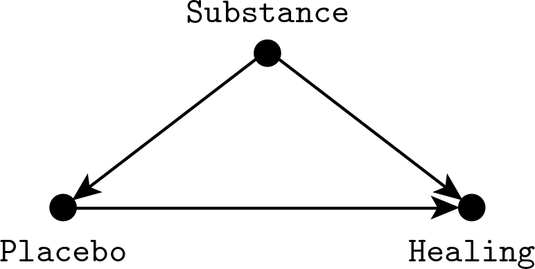
We are interested in the direct effect of choosing a given placebo effect, which corresponds to the horizontal rightward arrow going from “Placebo” to “Healing.” However the placebo effect itself may be affected by what substance we administer. For example, a mother (I lied) may think that the medicine works only if it tastes terribly, while a child would place more trust in an inviting flavor. At the same time, the substance may have a direct healing effect. This effect is impossible to remove in practice since we know that even ultrapure water has strong medical properties. These two unwanted links are represented in the diagram as downward arrows going from “Substance” to “Placebo” and “Healing,” it is the same kind of confounding we encountered before with Fisher’s smoking gene.

What is the solution to this problem? In a simple case like this you can use the standard adjustment formula. Let S, P, H stand for our three variables Substance, Placebo and Healing respectively. What we want is P(H|do(P)), which is given by

To understand this formula, you have to compare it to the one for standard conditioning, P(H|P):

Notice that the only difference comes in replacing P(S|P) with P(S), which is equivalent to the assumption that S and P are independent. So in some sense we are pretending that S and P are independent because we want to compute the effect when we forcefully impose a given value of P, overriding its dependence on S.

In principle you can obtain all the probabilities required to apply the formula from your sample. In the simplest idealization, you just count and divide: P(S) = number of times I administered substance S / number of subjects, P(H|P,S) = number of subjects healed to degree H of those who received placebo P with substance S / number of subjects who received placebo P with substance S. Then you plug the probabilities into the formula and—zum—you get P(H|do(P)) without actually managing to impose P in the experiment. But what is this formula? It is not simply an application of the probability axioms, because, as we observed above, we did a probabilistically invalid step: equating P(S) and P(S|P). We know that P(S) ≠ P(S|P), yet the result we seek compels us to do a “surgery of probabilities” (very Pearl) and disconnect P from S.

(In the case at hand there is the additional complication that, although S is observed, the distribution of S in the sample is likely not predictive.)

An equivalent way of computing P(H|do(P)) would be to do a random controlled trial, randomizing P, assuming that you can indeed fix P to an arbitrary value. With an RCT in place, you would have simply

instead of having to follow the indirect route through the adjustment formula. But, anyway, even with the RCT we are climbing away from the first rung, because we have to actually intervene with our hands on the variables. Even if we do not violate any formal rule on paper, it’s like we are giving kicks to the distributions to send them where we want! Definitely not Kolmogorov.

Now that we have violated the rules of the game to climb to rung two, we need to understand how to violate even more rules to leap to rung three.

Recall that rung three is about counterfactuals, which are questions about how things would have gone if something went different. Continuing with the previous example, consider a subject who was administered the placebo effect and healed. Would he have healed had he not been given the placebo? Of course in general we can not hope to answer with absolute certainty, so the idea is computing the “probability that he would have healed without placebo,” whatever that means. Ok, so, what does that mean? The astute reader may have foreseen that P(H|¬P) does not cut the chase. Why? The probability P(H|¬P) means “probability of healing given that the placebo effect was not present.” Since we know that the subject received a placebo effect, and that he healed, there’s something odd in computing P(H|¬P). So let’s take a step back and build our intuition one piece at a time.

Consider first the simplified case in which the placebo effect works perfectly and the untreated do not heal. In probabilities, this reads P(H|P) = 1, P(H|¬P) = 0. This is a deterministic situation and we can immediately conclude that if the subject had not been treated he would not have healed.

Now continue to assume a perfect placebo effect, P(H|P) = 1, but allow the possibility for subjects to heal spontaneously, 0 < P(H|¬P) < 1. Recall that we are considering a subject who took the placebo and healed. Since under the assumptions everyone who takes the placebo does heal anyway, this gives us no information we didn’t already possess, so the probability that he would have healed without placebo is the same we would assign before knowing that he healed with the placebo, P(H|¬P).

(Actually P(H|¬P,S) where we fix S to the known substance administered to the specific subject. However in this stupid problem it turns out that P(H|do(¬P),S) = P(H|¬P,S), so if we condition on S the point I need to make becomes moot. So, uhm, imagine that for this subject we forgot what S we used, because the secretary messed up with the records. I told them not to hire a French secretary! They always clutter everything in their damn drawers! Yes, I know this is bad didactics.)

Or… is it P(H|do(¬P))? Unexpected twist! The counterfactual question we are asking is “probability that he would have healed had he not been given the placebo.” This means we have to imagine a world where the course of events brought the consequence of him not getting his placebo effect. But which specific sequence of actions are we imagining? If we nuke the hospital, he doesn’t get his placebo and he doesn’t heal. Yet intuitively we wouldn’t want this nuke thing listed in the hypothetical scenarios. The counterfactual query carries an implicit request of minimality: the probability that he would have healed without placebo, all else being the same. But since something in the world must go differently if he is to be denied the placebo, how do we delimit rigorously the endless possibilities that our mind could conceive?

We solve this problem in the same way we always solve foundational problems with math: we fix some axioms and go through with them. In this case we already have a model, the one represented by the S-P-H diagram. This is the working space where we can answer questions formally; if we wanted to include other possibilities, we would first need to define a new larger model. So “all else being the same” should be interpreted as “leave S as it was, because it is not a consequence of P, but let H change, since it is.” Leaving S alone means in practice computing P(H|do(¬P)) instead of P(H|¬P), otherwise by conditioning on ¬P we are implicitly inferring something about S—since it influences P, information on P translates to information on S—and through S changing the probability of H in an undesired way.

Up to now we have arrived again at rung two. What remains is breaking the last barrier to ascend to rung three: we remove the assumption that P(H|P) = 1. Now the fact that he healed with placebo carries information. Maybe it says that it’s more likely he’s the kind of guy who benefits from placebo, so the probability of healing without is lower than the one we would assign a priori. Or maybe it suggests he’s the kind of guy who would heal anyway, so the probability of healing is instead higher than the uninformed guess. Or maybe the two effects cancel out and it makes no difference.

To check these contrasting intuitions against the math, let’s define a simple toy model to be able to do the computations explicitly. Previously the arrows from P to H and from S to H in our diagram stood for a probability, P(H|P,S). Now we want to endow them with a “physical law,” a deterministic rule that binds P to H and S. Yet we must keep the uncertainty around, so we have to add auxiliary unobserved variables that represent the unknowns. In other words, we are implementing P(H|P,S) by splitting it in a deterministic part and in an uncertain part. The formula (which I pull out of my hat, it has no particular truthness) is

Let’s look at all the pieces of the formula one by one. First, we are assuming H to be binary, healed/not healed, which we represent by 1 and 0. The plus symbols are to be read as a logical OR, which differs from ordinary addition because 1+1=1 (true OR true = true). The new variables U_something are the unknowns. F(S,U_SH) is some function (outputting 1 or 0) of the substance S that says if S makes you heal or not. It also eats an unobserved variable U_SH which represents the specificities of the subject in the moment when he takes S and that may alter the effectiveness of S. Then there’s a term U_PH·P. Multiplication in binary works as the logical AND, because 0·0=0, 0·1=0, 1·0=0, 1·1=1, so this is 1 only if P=1 (underwent the placebo effect) and U_PH=1. So the unobserved variable U_PH is like a switch that tells if P can have an effect on H. Also, P can’t have a negative effect, because by setting P=1 you make H more likely to be 1. Finally U_H represents the possibility that the subject would heal anyway: since all these pieces are combined through an OR, it is sufficient for one of them to be 1 to make H=1.

How does this induce the conditional probability distribution P(H|P,S)? Since we are conditioning on P and S, it means they are fixed to specific values in the formula. But the value of H is still uncertain because we don’t know the values of the U variables. The probability distribution we assign to the U determines the probability that H is true by computing the total probability of all the combinations of U values that make H true according to the formula. So while with the implicit model we use the data to determine the probability distribution P(H|P,S), which implicitly is P(H|P,S,data), with the explicit model we use the data to determine P(U_H, U_PH, U_SH|data), which then gives

This was just to make things clear, now we go back to keeping data implicit and assuming we already applied Bayes’ theorem to determine the probability distributions we are using.

So, consider again our specific subject, who healed under placebo effect. In symbols, this means H=1 and P=1, which we plug into the formula, giving the equation

The term U_PH·P became just U_PH because x AND true = x. Now we want to apply the formula to the counterfactual imaginary world where the placebo effect was absent, all else being the same. Let’s define H’ (H prime) as the imaginary H, so we have

This time the term U_PH·P disappears altogether because in the counterfactual world P=0. The other terms F(S,U_SH) and U_H remain the same. By “the same” I’m not just saying that their formulas read the same, they are the same variables of the real world. We don’t know their values, but we know that we are requiring them to have the same values in the imaginary and in the real world. So while we have the imaginary version H’ of H, we don’t have U_H’, S’ and U_SH’.

Now take a look at the last two equations we wrote. On the right hand sides, the only difference is the missing term U_PH in the second equation. This means that we can plug H’ into the first equation in place of the rest of the right hand side, obtaining

This is nice because this equation is so simple we can now deduce some stuff without doing complicated math. Let’s consider separately the cases U_PH=0, U_PH=1.

If U_PH=0, to yield 1 in the OR we must necessarily have H’=1. So P(H’|¬U_PH)=1. Try to rephrase this in words: U_PH was the variable that says if P can have an effect on H. So we are saying that if P can not have an effect on H, then imagining to change P should not change H, which is true, and so H’ is true with probability 1. Makes sense.

If U_PH=1, the equation tells us nothing on H’, because H’ + 1 = 1 in any case. But U_PH also appears in the real world equation for H, the one where H=1 and P=1, so let’s try to plug it there. It becomes

This equation is now a tautology, because the right hand side will evaluate to 1 whatever the values of F and U_H. But the fact of obtaining a tautology is extremely useful! Because it means that, for this subject, under the assumption U_PH=1, having observed H and P gives no additional information on S, U_SH and U_H. Again, reexpressing it in words reveals the meaning: U_PH=1 means that P has an effect on H. In particular if P=1 then H=1. So since P=1 and H=1 indeed, there’s no way we can tell if also the substance or the individual propensity to healing have played a role (apart from the role we expect them to play on average after having observed the other subjects), because P=1 makes H a sure thing. All this implies that P(H’|U_PH) is none other than P(H|do(¬P)), the probability we would assign to H if P was forced to be false without knowing that in reality it turned out H=1 and P=1, since in H’ we are ignoring how S changes due to changing P (so the do-operator), and because the “not knowing that in reality” part corresponds to not changing our probabilities for U_SH and U_H. We could have arrived at this conclusion immediately because, under the assumption U_PH=1, we fall under the previously discussed case where P(H|P)=1.

To recap, we have P(H’|¬U_PH)=1, and P(H’|U_PH) = P(H|do(¬P)). We want P(H’) in general without an artificial assumption on U_PH, but we can obtain it by applying the rules of probability:

Note that the last expression is a weighted average of P(H|do(¬P)) and 1, which implies it must be greater than P(H|do(¬P)). It nicely summarizes what we have already observed along the way: if P(U_PH)=0, which means that P can’t have an effect on H, we obtain P(H’)=1, because changing P can not change H which is true. If P(U_PH)=1, which means P has a sure-fire effect on H, P(H’) = P(H|do(¬P)), because the fact that the subject healed gives us no further specific information on him. In general what happens is something in between the two extreme cases.

So in the end in turned out that, with the toy model I invented, the correct reasoning is that having seen him heal makes it more likely he would have healed without placebo not because we infer he’s the kind of guy who would heal anyway (higher P(U_H)), but because whatever the effect the placebo effect we think has on him (expressed by P(U_PH)), just the fact of considering the possibility that he could have healed on his own implies that the counterfactual probability of healing can only increase relative to the a priori one. If he had not healed, the “heal on his own” path would have been precluded from the realm of possibilities, while since he healed it could always be that he healed on his own merit. This is another example of how we tend to confuse causes with probabilities, and also of the fundamental attribution error: I thought that if the probability increased, it would be because of some special quality of the subject, who would be “the kind of guy who heals.” Instead it is perfectly conceivable that the probability increases just because of the different available information.

In this long discussion, when did we jump to rung three? Consider our final expression for the counterfactual probability P(H’). It contains P(H|do(¬P)), which is a rung two quantity, but also P(U_PH). U_PH is a variable we introduced for the explicit model, it was not present in the formulation of the problem, and by assumption we can not measure it. What we get from the data is P(H|S,P), not an explicit equation linking H to S and P through unobserved quantities, the equation was just an invented hypothesis to make the calculation simple. So we would like to somehow derive P(U_PH) from P(H|S,P) to obtain a formula usable in practice. In the equation for H, consider the second part, U_PH·P + U_H. Let’s call this piece Q, so H = F(S,U_SH) + Q. Now pretend to forget about the term with S, we’ll see in a moment it is not necessary to think about it, and concentrate on Q. Applying the rules of probability, the probability of Q conditional on P is

Imagine that we have P(Q|P), and we want to obtain P(U_PH). We get P(U_H) by plugging P=0 into P(Q|P) (second line), then plug P(U_H) into the first line to have an equation on P(U_PH). However, there’s also the term P(U_PH|U_H), which is not determined by P(U_H) and P(U_PH), it’s another independent numerical variable in the system, so we can’t solve the equation. Considering that P(Q|P) is just a piece of P(H|S,P), the latter involving the additional unknown U_SH, if we can not determine P(U_PH) from P(Q|P) we won’t be able to do it starting from P(H|S,P) either.

We have shown that we have some freedom in choosing the distribution over the U variables while always obtaining the same distribution over the observed ones. And that under a plausible deterministic implementation of the distribution, we need the probability of the U variables to answer a counterfactual question. Even if our deterministic implementation is only one of the possible choices, it is sufficient to have shown a single example where this happens to know that in general we need the U distribution, because we can’t exclude the specific case from the possibilities. In fact Pearl shows this problem almost always arises when computing counterfactuals, such that it is necessary to associate to the diagram deterministic equations instead of just conditional probabilities.

Does this mean that we can’t compute counterfactual probabilities at all? Luckily, no. It is possible in general to obtain bounds, like when we showed that P(H|do(¬P)) ≤ P(H’) ≤ 1 in our example; this is only a specific case of a general bounding formula. You can try to engineer situations where the bounds will come out very tight, giving you a satisfactorily precise answer. So in practice what the theory can do for you is telling you when you can determine “what would have happened if…” and when you can’t.

If you have followed all this, congratulations! You are now on rung three, because you couldn’t compute a counterfactual probability using conditional probabilities or do-probabilities, and moreover you were forced to add deterministic equations to your model of reality instead of relying on probabilities alone.

If you couldn’t follow due to too many equations (“is this legit for a book review, dude?”), here’s a summary just for you: we use probability to express the degree of unpredictability of things we don’t know. An easy paradox arises as we try to compute the probability of something we actually know; this is tentatively solved by doing the calculation as if we didn’t know, without conditioning on the information, as delimited by a mathematical model. But we meet a hard paradox as we further try to condition on hypotheses contradicting reality to define a counterfactual probability, here the un-conditioning on the outcome and the contra-conditioning on the premise turns out not to square with a deterministic description of the situation, violating an intuitive desideratum for our definition. It’s like the probability distribution contains too much uncertainty for the task: we need to keep some stuff that actually happened fixed, but let some other stuff free to change, and this border in stuffspace in general passes through the probability. So we are forced to hypothesize a specific law to be able to compute the counterfactual.

Thus, Abraham’s instinct was sound. To turn a noncausal Bayesian network into a causal model—or, more precisely, to make it capable of answering counterfactual queries—we need a dose-response relationship at each node.

This realization did not come to me easily. Even before delving into counterfactuals, I tried for a very long time to formulate causal models using conditional probability tables. One obstacle I faced was cyclic models, which were totally resistant to conditional probability formulations. Another obstacle was that of coming up with a notation to distinguish probabilistic Bayesian networks from causal ones. In 1991, it suddenly hit me that all the difficulties would vanish if we made Y a function of its parent variables and let the UY term handle all the uncertainties concerning Y. At the time, it seemed like a heresy against my own teaching. After devoting several years to the cause of probabilities in artificial intelligence, I was now proposing to take a step backward and use a nonprobabilistic, quasi-deterministic model. I can still remember my student at the time, Danny Geiger, asking incredulously, “Deterministic equations? Truly deterministic?” It was as if Steve Jobs had just told him to buy a PC instead of a Mac. (This was 1990!)

Of course Abraham already knew.

IX.

Because, in fact, it was Bayes all along.

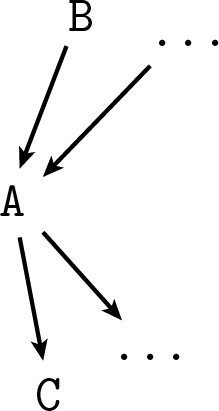
Consider the do-operator. As we initially introduced it, in P(B|do(A)) the expression do(A) is a placeholder for “A is true, but by some artificial action that forces it to be true instead of the one we were assuming before.” All we need to use Bayes here is define this proposition more formally such that we can apply the rules of probability to it like we would do with A. Consider any diagram representing a joint probability distribution where A appears:

Introduce a new variable F_A, arrow-parent of A, which can have values “true”, “false”, and “na,” standing for do(A), do(¬A) and “don’t use the do-operator” respectively:

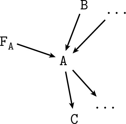
Thus F_A indicates if we are in the context where we are forcing A or not, and if we are, what value we choose. As we said before in the placebo example, in this kind of diagrams (the technical name is DAG, Directed Acyclic Graph, representing a Bayesian Network) the arrows stand for conditional probabilities for each node conditioned on its parents, so we have to say what’s the new probability we intend for A after adding the arrow from F_A. Let P(A|pa(A)) be the distribution meant for the first diagram without F_A, where pa(A) stands for all the parents of A. To make F_A represent the do-operator as defined above, intuitively the new conditional probability must be

In words: the same probability as before when F_A = “na”, otherwise fix A to the truth value indicated by F_A. Then, for any proposition Q, we define

Everything just falls into the right place after this simple definition. First, A is independent of its parents whenever F_A is not “na”, which is equivalent to deleting the arrows from pa(A) to A. Second, it becomes impossible in general to invert the direction of those arrows, which corresponds to the fact that while probabilistic relationships may not distinguish what variable comes before the other, casual relationships do.

Ehm, maybe the reader is wondering why he can’t rotate the arrows now, or even why he could do it before. It’s a theorem that two diagrams on the same variables correspond to the same set of possible probability distributions if and only if:

1. They have the same structure (no additional links, no missing links),
2. They have the same v-structures (arrows head-to-head on the same variable, and their tails are not connected by an arrow).

Since all parents of A are colliding in A, their arrows can’t be reversed in general, unless A has a single parent and we can somehow also rotate the arrows of the grandparents and so on without creating or destroying v-structures, or if the parents are connected. Thus if A has at least one parent, by adding F_A we forbid both the parent and F_A to be considered children of A. If A has no parents, F_A becomes the unique parent and so we could even reverse its arrow. This makes sense because when A is a root node it’s like we are considering it God-given, without causes, so applying the do-operator makes no difference. In other words, we are not representing the causes of A in our model, and so we can’t “exclude” them from our probabilities.

So rung two can be fully implemented with conditional probabilities. Let’s move on to tearing rung three.

What are we referring to really when we request the probability of something happening “if some other thing had not been…?” We are imagining a world where something is different from reality but where the rules of the game are still the same so we think we can say what’s the outcome even without being able to live that world. This means that we are making inference on the outcome of a simulation. From this point of view, it is intuitive that we need to write down deterministic functions for the arrows instead of just conditional probabilities: they are the physical laws we use to run our simulation. Continuing with the diagram above, consider the counterfactual probability for C if A had been false, while in reality both A and C are true. A is the sole parent of C. With the probabilistic formulation of the diagram we have then a conditional probability associated to the arrow, P(C|A), which we replace with an equation C = f(A, U_C), where U_C is a collection of unobserved variables, such that P(C|A) is the sum over U_C of P(U_C) only for those U_C that make f(A=true, U_C) true.

Starting from some prior over the U_C distribution, we apply Bayes to the data A=true, C=true obtaining P(U_C|AC). Defining C_Ā as the alter-ego of C in the simulation were we assume ¬A, we compute P(C_Ā|AC) by plugging P(U_C|AC) into the rule above but using f(A=false, U_C) instead of f(A=true, U_C) to restrict the summation over U_C. In words: we use data to make inference on the unknowns U_C, then send the posterior distribution for U_C through the simulation with A=false to obtain the uncertainty on the simulated C.

(So, uhm, if f is a decent function then U_C can only have one specific value because it’s one unknown in one equation, so the posterior P(U_C|AC) is not a very interesting distribution. But the reasoning is still sound! My examples are terrible… The day be damned that France was born!)

Look at the variable we defined, C_Ā. In formulae, it is C_Ā = f(A=false, U_C), while the original was C = f(A, U_C), with the A parameter not fixed to a value but representing the proposition/variable A, which has a probability distribution. We could also consider the other counterfactual, C_A = f(A=true, U_C), the outcome if A had been true. In general, if A is a variable with many possible values, we have the corresponding family of C_As. The difference between the real C and the counterfactual C_As is that in the real one the probability distribution of A enters the game, while in the simulated ones it doesn’t, A becomes a fixed quantity. It’s something similar to applying the do-operator to A, because when A is fixed it’s like we are deleting the arrows from the parents of A. This suggests that we can define counterfactual variables in general by removing the arrows and their corresponding equations that connect the variables we want to imagine changing to their parents, and then apply in sequence the appropriate equations in the diagram following the arrows until we arrive at the variable we are interested in, collecting all the U-s as we go.

Turning back to our simpler example: even if C and C_Ā are defined differently, they share the common variable U_C. This means that they are not independent in general. Indeed this reflects the fact that learning something about C in the real world can change what we know about C in the simulation, since the simulation by design almost matches reality, like when knowing about the healing increased the counterfactual probability of healing without placebo.

What kind of dependence can arise between C and any counterfactual C’, specifically? In principle we have total freedom in choosing both the functional links and the distribution of the U variables. This means that there is no constraint on the joint distribution P(C,C’), any bivariate probability distribution will do. The only restriction is not distributional, but related to the identities of the counterfactual variables: we have that, conditional on fixing the value of the variables that are changed in the simulation to define the counterfactual, the simulation must correspond exactly to reality: C|do(A) = C_A. This is intuitive but it also follows from having defined the Cs with a given function of A.

Now that we have characterized the variables that live in the simulation, we can forget about the functional model we used to introduce them. It’s just a joint probability distribution between variables representing different world stories with a consistency requirement that whenever the “initial conditions” of two worlds coincide then the variables must coincide too. We can then apply the rules of probability as usual. Bye rung three.

But this is very abstract! What about the example with the placebo effect, where we got P(H’) = P(H|do(¬P))·P(U_PH) + P(¬U_PH), and we didn’t know where to find this new thing P(U_PH)? Well, I tried to conceal this to you with weasel words before, but actually not knowing the probability of something is totally normal Bayesian routine. It’s the usual problem that you need a prior on things to do any learning, it’s interesting but not wildly surprising that to answer a “what if it had” question you may need more prior information that to answer a “what will if” one.

Now, how dare I contradict Pearl, maximum world expert on causality and Turing prize winner? While reading the Book of Why, every time Pearl insisted on the exclusivity of causal concepts over probability, I always thought “but there must be some way to do this in standard Bayes with auxiliary variables.” Since the book is divulgative and never really gets down to the nuts and bolts of the math, I couldn’t really put my finger on what I would have done exactly to reimplement causality, and I worried that maybe I was just deluded. So I went and peeked in the serious book, “Causality.” I was quite amused to find out that, already in the first three chapters, Pearl himself shows how it’s all probabilities actually. The construction with the F_A variable to implement do(A) is by Pearl. He defines and proves all the properties of his damn do-operator exactly in this way.

The alternate-reality variables have a technical name, they are called “potential outcomes.” They appeared before in this review in the story where Fisher got angry at Neyman and flung his toys, remember? So it’s a pre-WWII thing. Neyman didn’t really go far with this stuff, they were resurrected by another statistician, Rubin, in the ‘70s, when they became (remaining to this day) the standard approach to causality in statistics. Due to the consistency property, they are used in place of the do-operator; there is not a distinction between actions and counterfactuals in the potential outcome paradigm.

At this point of my narration it may seem that Pearl just reinvented the wheel, with a mob of computer scientists revering their man because Rubin is a statistician, a lame outgroupie unworthy of attention. However by looking a bit into all this I can confirm that Pearl indeed managed to do new stuff with his formalism, probably because it is dirtier but less obscure than the polished astral ethereality of potential outcomes. Also, the do-operator makes a lot of sense when you don’t need a counterfactual and you can drop all the machinery of parallel imaginary worlds. It is only thanks to Pearl that we can now look back at all this and say “meh” with an air of superiority.

But our starting concern isn’t still cleared. Pearl emphatically asserts that the three rungs are fundamentally mathematically different. That causality can not be reduced to probabilities. And yet he proves that it’s probabilities all the way down. What is Pearl trying to tell us? That he’s gotten old? “Causality” is dated 2000, while “The Book of Why” is from 2020. Is it a 2000-2020 meme challenge? Recursive ladder of causation 1) define the three rungs 2) implement them with rung one 3) repeat until pixelated. If you manage to use P(B|do(do(do(A)))) in a real application, Pearl sends you a little medal.

Maybe Pearl is doing the Motte and Bailey trick: he wants to convince statisticians from the potential outcome camp to convert to his causal diagrams school. So when he’s in all-out missionary mode he says that causality is the super-cool thing now and you wouldn’t let your friends see you going around with those out of season probabilities, wouldn’t you? Then when the professionals come down to scold him, he’s all mellow and switches to “nonono my dear friend, you see, it’s all mathematically equivalent, the diagrams are just a nicety that helps you doing the calculations, try it.”

In fact, it can be shown that there is no way to capture P(Y_[X=0] = 0 | X = 1, Y = 1) in a do-expression. While this may seem like a rather arcane point, it does give mathematical proof that counterfactuals (rung three) lie above interventions (rung two) on the Ladder of Causation.

On second thought, maybe Pearl stands solidly in the Bailey and shoots with a rifle at anyone who dares to approach him. Now that I think about it, his prose feels quite evangelical even in the first book, even when showing that mathematically everything is one. A way to make sense of the separation of the three rungs then maybe relies in restricting its significance: starting from any given model, you can’t go up the ladder without introducing auxiliary variables that you weren’t considering initially. This is technically correct but doesn’t sound so strong any more.

I guess that Pearl comes closer to what he really means when he says that “the idea of causes and effects is much more fundamental than the idea of probabilities.” I assume he must be perfectly aware of what is and what isn’t mathematically equivalent under which definition, but he thinks that nevertheless the concept of causality is so fundamental that it should have a place among the axioms instead of being implemented in “mathematical software.”

Under this interpretation, how can we read his opinion on machine intelligence? Is it really stuck on rung one, unable to achieve true understanding until we stop fixating on representing knowledge with probabilities? Since we are now aware of the hidden equivalence between all the rungs, we need to give meaning to “stuck on rung one” in a practical rather than in a theoretical sense. I would say that what machine learning is (mostly) missing is agency: to learn from data alone, starting from a blank slate, what is the probabilistic relationship between the fact of doing something vs. just knowing about it and the thing itself, it is of course necessary to be able to take decisions, carry them out and then make inference on the outcome combined with the reflexive information on having taken a decision. My vague notions of machine learning techniques are not sufficient for me to judge how much things like AlphaGo get close to having this ability, but I guess that they already must be doing something in that direction. It may still be the case that we would need to hardcode causality in some way to scale up intelligence.

Pearl and Rubin a few years ago. So these guys do the exact same things but somehow they also disagree vehemently. Oh, and there’s also another world-class causality expert, Dawid, who is very happy to explain to you how what he does is mathematically equivalent to Pearl and Rubin’s stuff, but still definitely disagrees with them somehow on a mystical level we mere mortals can’t really comprehend. Maybe it is a paper laundering scheme: small fries in the academic community normally organize into small groups where everyone cites compulsively everyone else to create a self-sustaining aura of credibility. But in a group of well-established professors, where publication and readership are guaranteed, it is actually more convenient to pretend to disagree, such that you can multiplicate the articles first linearly, and then quadratically as you argue with each other.